


13
Electroencephalography
 Spontaneous
activity is measured on the scalp or on the brain and is called the
electroencephalogram. The amplitude of the EEG is about 100 µV when
measured on the scalp, and about 1-2 mV when measured on the surface of
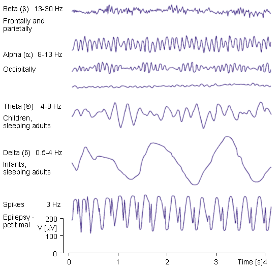
the brain. The bandwidth of this signal is from under 1 Hz to about 50
Hz, as demonstrated in Figure 13.1. As the phrase "spontaneous activity"
implies, this activity goes on continuously in the living individual.
Evoked potentials
are those components of the EEG that arise in response to a stimulus
(which may be electric, auditory, visual, etc.) Such signals are usually
below the noise level and thus not readily distinguished, and one must
use a train of stimuli and signal averaging to improve the
signal-to-noise ratio.
Single-neuron
behavior can be examined through the use of microelectrodes which impale
the cells of interest. Through studies of the single cell, one hopes to
build models of cell networks that will reflect actual tissue
properties.
Spontaneous
activity is measured on the scalp or on the brain and is called the
electroencephalogram. The amplitude of the EEG is about 100 µV when
measured on the scalp, and about 1-2 mV when measured on the surface of
the brain. The bandwidth of this signal is from under 1 Hz to about 50
Hz, as demonstrated in Figure 13.1. As the phrase "spontaneous activity"
implies, this activity goes on continuously in the living individual.
Evoked potentials
are those components of the EEG that arise in response to a stimulus
(which may be electric, auditory, visual, etc.) Such signals are usually
below the noise level and thus not readily distinguished, and one must
use a train of stimuli and signal averaging to improve the
signal-to-noise ratio.
Single-neuron
behavior can be examined through the use of microelectrodes which impale
the cells of interest. Through studies of the single cell, one hopes to
build models of cell networks that will reflect actual tissue
properties.
 i (volume source)
 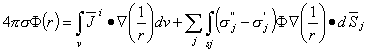 | (13.01) |
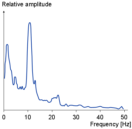
Fig. 13.1. Frequency spectrum of normal EEG.
In addition to the 21
electrodes of the international 10-20 system, intermediate 10% electrode
positions are also used. The locations and nomenclature of these
electrodes are standardized by the American Electroencephalographic
Society (Sharbrough et al., 1991; see Figure 13.2C). In this
recommendation, four electrodes have different names compared to the
10-20 system; these are T7, T8, P7, and
P8. These electrodes are drawn black with white text in the
figure.
Besides the international
10-20 system, many other electrode systems exist for recording electric
potentials on the scalp. The Queen Square system of electrode
placement has been proposed as a standard in recording the pattern of
evoked potentials in clinical testings (Blumhardt et al., 1977).
Bipolar or unipolar
electrodes can be used in the EEG measurement. In the first method the
potential difference between a pair of electrodes is measured. In the
latter method the potential of each electrode is compared either to a
neutral electrode or to the average of all electrodes (see Figure 13.3).
The most recent guidelines
for EEG-recording are published in (Gilmore, 1994).
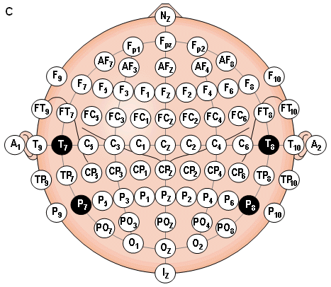
Fig. 13.2. The international 10-20 system seen from (A) left and
(B) above the head. A = Ear lobe,
C = central, Pg = nasopharyngeal,
P = parietal, F = frontal,
Fp = frontal polar, O = occipital.
(C) Location and nomenclature of the intermediate 10% electrodes, as
standardized by the American Electroencephalographic Society. (Redrawn
from Sharbrough, 1991.).
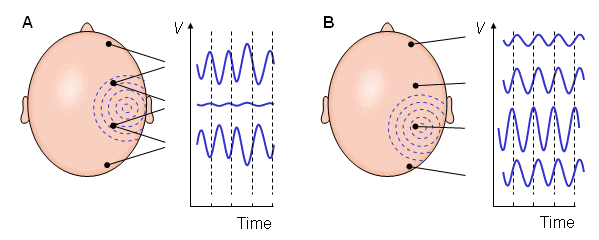
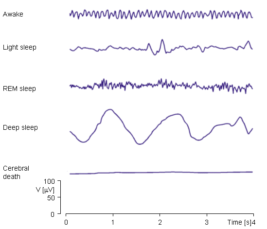
Fig. 13.3. (A) Bipolar and (B) unipolar measurements. Note that the waveform of the EEG depends on the measurement location.
Puikkonen and Malmivuo
(1987) recalculated the sensitivity distribution of EEG electrodes with
the same model as Rush and Driscoll, but they presented the results with
the lead field current flow lines instead of the isopotential lines of
the lead field. This display is illustrative since it is easy to find
the direction of the sensitivity from the lead field current flow lines.
Also the magnitude of the sensitivity can be seen from the density of
the flow lines. A minor problem in this display is that because the lead
field current distributes both in the plane of the illustration as well
as in the plane normal to it, part of the flow lines must break in
order to illustrate correctly the current density with the flow line
density in a three-dimensional problem. Suihko, Malmivuo and Eskola
(1993) calculated further the isosensitivity lines and the half-sensitivity
volume for the electric leads. As discussed in Section 11.6.1, the
concept half-sensitivity volume denotes the area where the lead field
current density is at least one half from its maximum value. Thus this
concept is a figure of merit to describe how concentrated the
sensitivity distribution of the lead is. As discussed in Section 11.6.6,
when the conductivity is isotropic, as it is in this head model, the
isosensitivity lines equal to the isofield lines of the (reciprocal)
electric field. If the lead would exhibit such a symmetry that adjacent
isopotential surfaces would be a constant distance apart, the
isosensitivity lines would coincide with the isopotential lines. That is
not the case in the leads of Figure 13.4.
Figure 13.4 displays the
lead field current flow lines, isosensitivity lines and half-sensitivity
volumes for the spherical head model with the electrodes located within
180°, 120°, 60°, 40°, and 20° angles. Note that in each case the two
electrodes are connected with 10 continuous lead field flow lines.
Between them are three flow lines which are broken from the center,
indicating that the lead field current distributes also in the plane
normal to the paper. The figure shows clearly the strong effect of the
poorly conducting skull to the lead field. Though in a homogeneous model
the sensitivity would be highly concentrated at the electrodes, in the
180° case the skull allows the sensitivity to be very homogeneously
distributed throughout the brain region. The closer the electrodes are
to each other, the smaller the part of the sensitivity that locates
within the brain region. Locating the electrodes closer and closer to
each other causes the lead field current to flow more and more within
the skin region, decreasing the sensitivity to the brain region and
increasing the noise.
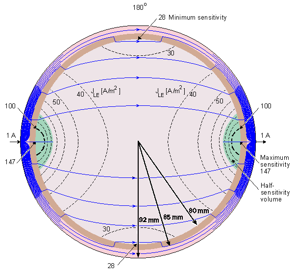
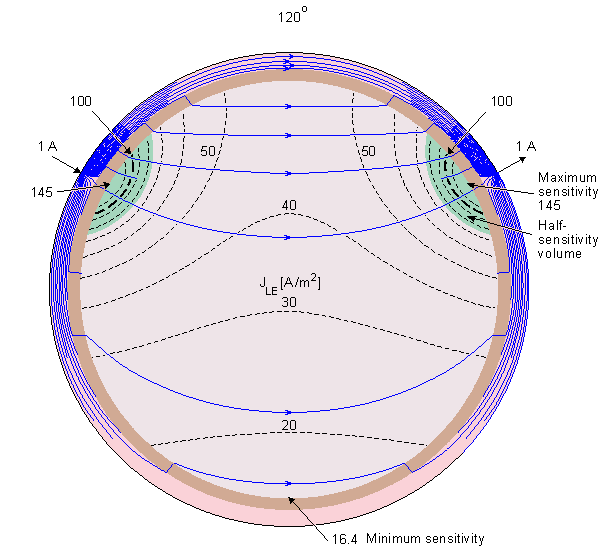
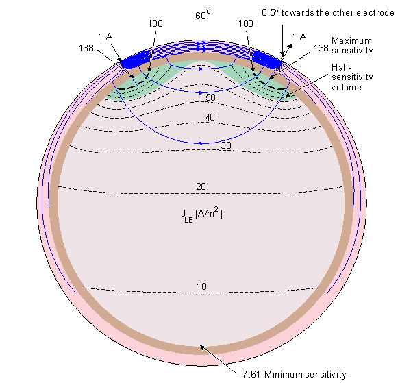
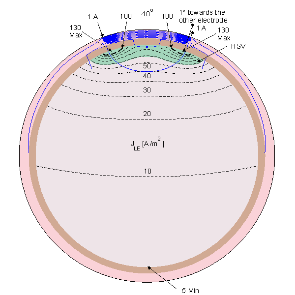
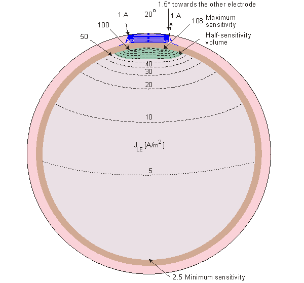
Fig. 13.4. Sensitivity distribution of EEG electrodes in the spherical head model. The figure illustrates the lead field current flow lines (thin solid lines), isosensitivity lines (dotted lines) and the half-sensitivity volumes (shaded region). The sensitivity distribution is in the direction of the flow lines, and its magnitude is proportional to the density of the flow lines. The lead pair are designated by small arrows at the surface of the scalp and are separated by an angle of 180°, 120°, 60°, 40°, and 20° shown at the top of each figure.
The alpha waves have the
frequency spectrum of 8-13 Hz and can be measured from the occipital
region in an awake person when the eyes are closed. The frequency band
of the beta waves is 13-30 Hz; these are detectable over the parietal
and frontal lobes. The delta waves have the frequency range of 0.5-4 Hz
and are detectable in infants and sleeping adults. The theta waves have
the frequency range of 4-8 Hz and are obtained from children and
sleeping adults..
Berger H (1929): Über das Elektroenkephalogram des Menschen. Arch. f. Psychiat. 87: 527-70.
Cooper R, Osselton JW, Shaw JC (1969): EEG Technology, 2nd ed., 275 pp. Butterworths, London.